Architecture Overview
Openwit is a high-performance OLAP (Online Analytical Processing) database designed specifically for observability data – namely logs, traces, and metrics. It is built with a focus on fast data ingestion, real-time query processing, and scalability.
Openwit’s architecture leverages a Rust-based actor system for robust, non-blocking concurrency. This means the system can handle many tasks in parallel without slowing down, which is ideal for the high volume of data in observability use-cases.
A key aspect of Openwit is flexibility in deployment:
- It can run in a Monolithic Mode (all components in one process on a single server for simplicity).
- It can scale out in a Distributed Mode (multiple specialized nodes working together in a cluster).
All behavior and settings are controlled via a unified configuration file (e.g., openwit_unified_control.yaml). In this config, you can tweak everything from what nodes to run, to batch sizes, file sizes, and other parameters, giving you complete control over the system’s operation.
In summary, Openwit aims to unify observability data handling (logs, metrics, traces) in one system that is easy to deploy in different modes, while ensuring high throughput ingest and lightning-fast queries. To truly understand how it achieves this, let’s break down its architecture and components.
Modes of Operation: Monolithic vs Distributed
Openwit can run in two modes, each suited to different needs:
Monolithic Mode: In this mode, all components run within a single node (server/process). Essentially, one machine hosts the entire Openwit system. All the functional elements (ingestion, storage, search, etc.) operate within a single application. They communicate internally (in-process) but conceptually act as separate logical parts. Monolithic mode is useful for development, testing, or smaller deployments, since it’s simpler to set up – everything is contained in one place.
Distributed Mode: In this mode, different components run on different nodes (servers/processes) and work together over a network. Openwit breaks its functionality into multiple specialized node types (up to nine, explained below). Each node type handles a specific responsibility in the pipeline. In a cluster, you might have multiple instances of some node types (for scalability or redundancy). Distributed mode is meant for high-scale scenarios where you need to ingest and query large volumes of data efficiently by spreading work across many machines.
Node Types in Distributed Mode
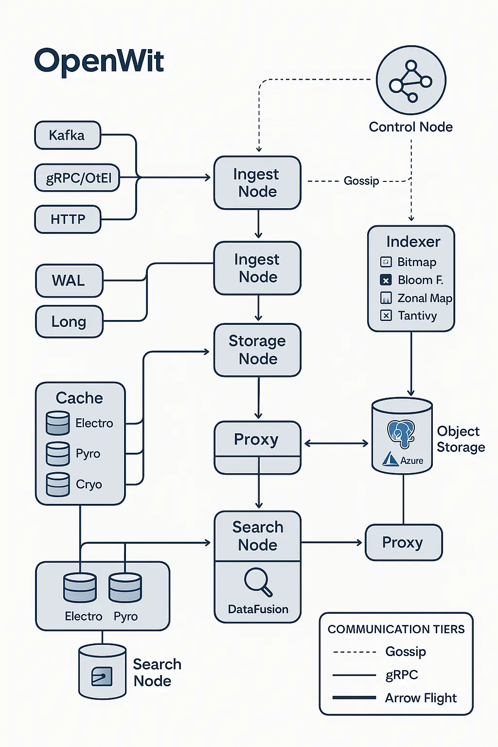
Openwit’s distributed architecture includes the following nine node types, each with a dedicated role:
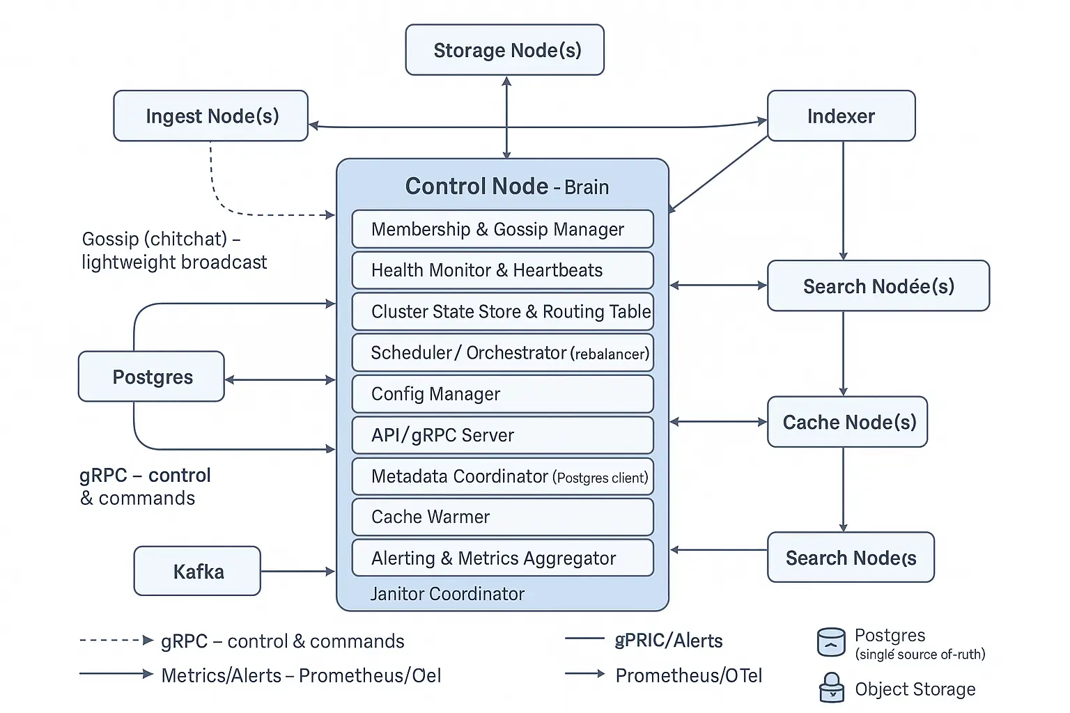
Control Node: The “brain” of the cluster, acting like a control tower. It keeps track of all other nodes, their status, and coordinates the cluster (which nodes should do what). If a node goes down or a new one joins, the control node orchestrates adjustments. It doesn’t handle data directly but manages everything else.
Ingest Node: Responsible for receiving batches of incoming data (after initial intake) and processing them for storage. It handles things like deduplicating entries, writing to the Write-Ahead Log (WAL), and forwarding data to storage nodes.
Kafka Ingest Node: A specialized node (or component) for ingesting data from Kafka streams. It pulls observability data from configured Kafka topics (streams of logs/metrics/traces) and feeds it into the pipeline.
gRPC Ingest Node: A node that accepts data via gRPC calls. This covers two cases – one using the standard OpenTelemetry gRPC format (so you can use existing OTEL exporters to send data to Openwit), and one for custom gRPC ingestion (if you define your own data proto and want to push data in a custom way).
HTTP Ingest Node: A node exposing an HTTP endpoint to receive data (in OTLP JSON or similar schema for logs, metrics, traces). This is mainly used for simplicity or testing – you can POST data directly over HTTP to see it flow through the system. (It’s not typically used for high-volume production data, but it’s handy for quick checks or simple integrations.)
Storage Node: Handles persistence of data to long-term storage. It collects processed data (in columnar format) from ingest nodes, buffers it into files (Parquet files), and uploads these files to cloud storage. It also triggers index creation for the data to enable fast search.
Proxy Node: Acts as an entry point or load balancer for the cluster. For example, clients might send queries to a proxy node, which then forwards the request to an appropriate search node. It can also route incoming data to the correct ingest node. (In essence, the proxy node helps external clients interact with a distributed cluster without needing to know each internal node’s address.)
Cache Node: Manages a cache of data for speeding up queries. It can store frequently queried data on local disk or in memory (configurable) to avoid repeatedly downloading data from the cloud storage. The cache node ensures that “hot” data is quickly accessible.
Search Node: The component that actually executes search and analytic queries. When you ask a question (SQL query) of Openwit, a search node is responsible for figuring out which data to read (with help from indexes and metadata), reading that data (possibly from cache or cloud), and computing the results to return to you.
In a distributed deployment, you might run several of each of these nodes depending on load: e.g., multiple ingest nodes if you have tons of incoming data, or multiple search nodes if you have many queries. The Control node ties it all together so the system works as one coherent whole.
Communication Between Nodes
In distributed mode, all these nodes need to communicate with each other. Openwit uses a three-layer communication strategy, choosing the right tool for the right type of message:
Gossip Protocol (via “Chitchat”): For small, frequent updates and broadcasts, Openwit uses a gossip protocol. Gossip is used to share lightweight state information with all nodes in the cluster. For example, things like: node health status (alive or not), node metadata (like “I am Node X of type Y on address Z”), small configuration details, etc.
These are usually not heavy data, but just small key-value info every node should know. Gossip is efficient for cluster-wide broadcasts without overloading any central point. Openwit leverages an implementation called Chitchat, which is a lightweight, robust gossip library. This way, every node eventually learns about the others (who’s in the cluster, who might have gone down, etc.) without needing a central monitor for health checks. Gossip updates are periodic and incremental, keeping overhead low.
gRPC Messages: For more direct, specific control instructions or medium-sized data exchanges, Openwit uses gRPC (Remote Procedure Calls). gRPC is a high-performance communication protocol (built on HTTP/2) that lets different parts of the system call each other’s functions as if they were local. In Openwit, many interactions that require a request-response or a targeted message use gRPC.
For instance, if an ingest node needs to ask the control node for configuration info, or a control node needs to instruct a specific storage node to flush data, these would be gRPC calls. gRPC messages are defined by protobuf schemas. Openwit has a set of protobuf definitions that cover these interactions. (In fact, the system provides default protobufs for common interactions like the standard OpenTelemetry data formats, and you can write new ones for custom interactions as needed.) gRPC is great for these scenarios because it’s efficient, typed (schema-based), and supports streaming if needed.
Arrow Flight for Bulk Data: When it comes to sending large volumes of data (like batches of logs/metrics/traces themselves), Openwit uses Apache Arrow Flight. Arrow Flight is a special high-speed data transfer protocol built on top of gRPC, designed specifically for sending large datasets in a performant way. Openwit converts incoming data into the Apache Arrow format (an in-memory columnar format) and then uses Arrow Flight to ship those Arrow record batches between nodes.
This is particularly used between the ingest nodes and storage nodes (to send big batches of data to be stored) and between storage/search nodes and cache/search nodes (to fetch data for queries). Arrow Flight is extremely fast because it’s binary, columnar, and can do zero-copy data transfers (meaning it doesn’t waste time serializing/deserializing or copying memory around unnecessarily). This makes sure that even heavy data loads (think millions of log lines or metrics) can be transferred across the network quickly and efficiently.
By combining these three communication layers, Openwit ensures that each kind of information is exchanged in an optimal way: cluster state is gossiped with minimal overhead, control signals are sent reliably with gRPC, and the heavy lifting of data movement is handled by Arrow Flight’s high throughput pipeline. This multi-layer design is one of Openwit’s advantages – it avoids using a one-size-fits-all network approach and thus achieves better performance and robustness.
Data Ingestion Pipeline
Now, let’s walk through how data enters Openwit and what happens to it. Openwit supports multiple ingestion methods to get observability data in:
Entry Points for Data
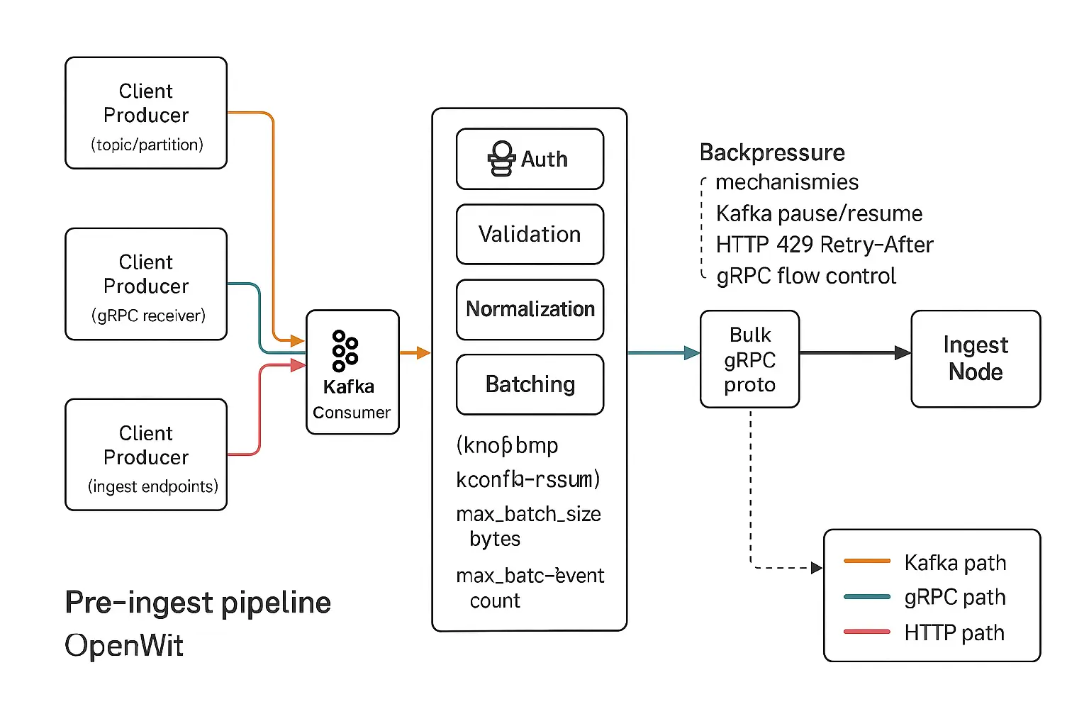
Kafka Ingestion: Kafka is a popular streaming platform often used to pipe logs and metrics from various sources. Openwit can ingest from Kafka by using the high-performance librdkafka library under the hood. You configure Openwit with your Kafka topic(s), and a Kafka ingest node will act as a consumer, continuously pulling messages. The incoming Kafka data (which in many observability setups is serialized in a binary format like Protobuf or JSON) is deserialized into Openwit’s internal data structures as the first step.
This deserialization is important because it converts raw Kafka bytes into structured objects (e.g., log events with fields, metric data points with timestamps and values), which Openwit can then process further. Kafka ingestion allows Openwit to seamlessly slot into an existing data pipeline where lots of data is already being pushed through Kafka.
gRPC Ingestion: Openwit offers gRPC interfaces for pushing data directly. There are two flavors:
- Standard OpenTelemetry gRPC: Openwit can natively understand and accept data from OpenTelemetry (OTel) exporters. OpenTelemetry has well-defined protobuf schemas for metrics, logs, and traces (often referred to as OTLP, the OpenTelemetry Protocol). If you have applications using OTel SDKs, they can export data via gRPC to Openwit without any custom work. Openwit’s gRPC ingest node uses prost (a Rust Protobuf implementation) and tonic (a Rust gRPC library) to handle these OTel messages. Essentially, this is plug-and-play for anyone already using the OpenTelemetry standards.
- Custom gRPC: In cases where the data format is not the standard, Openwit allows defining your own protobuf schemas and setting up a gRPC endpoint for them. For example, say you have a custom log format or an in-house metric structure; you can write a protobuf definition for it, and Openwit can incorporate that. You’d then send data to Openwit’s gRPC endpoint according to that schema. This requires a bit more work (writing and compiling the proto files), but it gives a lot of flexibility to integrate non-standard sources.
HTTP Ingestion: For quick tests or simple integration without needing a gRPC client, Openwit also provides an HTTP API. You can send an HTTP POST request with a payload containing observability data. The data can be in JSON (following the OpenTelemetry JSON schema for metrics, logs, or traces). The HTTP ingest node will accept these and push them into the system. This is very handy for trying things out manually (for example, using curl or a simple script to POST a log entry).
However, HTTP isn’t as well optimized for high throughput as Kafka or gRPC. In practice, the HTTP route is used to ensure the pipeline is working or for low-volume data; heavy production loads would use Kafka or gRPC for efficiency.
No matter which entry point data comes from, it converges into the same pipeline after this initial reception. Now we move to the Ingestion Gateway and Ingest Node, which handle the next stages.
Ingestion Gateway: Authentication, Validation, Batching
As data flows in from Kafka, gRPC, or HTTP, the Ingestion Gateway component is the first to process it within Openwit. Think of the ingestion gateway as a checkpoint that prepares and vets the data before handing it off deeper into the system. The ingestion gateway performs several crucial functions:
Authentication & Authorization: The gateway checks if the incoming data source is allowed to send data. For instance, if a client includes an auth token in the header, the gateway will verify it. This ensures that only authorized users or services push data into Openwit. It’s usually a simple token-based auth. If the token is valid, data proceeds; if not, it’s rejected. This provides a security layer right at the ingress.
Data Validation (Schema Enforcement): Observability data can be very heterogeneous (different services might send logs with different fields, metrics with different types, etc.). Openwit enforces a schema to maintain consistency. The gateway will validate incoming data against expected schema definitions:
- It checks that each field is of the expected data type. For example, if a schema says a certain field (say,
response_time) should be an integer, and some incoming data has it as a string "123" or a float123.45, that data point can be flagged or rejected. This prevents inconsistent typing that could cause errors or confusion later. - It ensures required fields are present and possibly drops unknown fields if they’re not in the schema.
By doing this, Openwit avoids the scenario where one service labels a metric or log field one way and another uses a different type for the same concept. All data will conform, making queries reliable (you won’t get mixed types in the same column, for instance).
Normalization (Consistent Naming): Even if types are correct, different sources might use different names for similar things. For example, one application might send a field called "user_id" and another might send "userid", or "status_code" vs "statusCode". The ingestion gateway tries to normalize these to a consistent schema. This could involve:
- Mapping known synonyms or variations to a standard name (perhaps via a configuration or a closest lexical match if it’s clearly the same concept).
- If it can’t find a logical match, the gateway might reject or log the discrepancy. The idea is to avoid subtle differences (like plural vs singular, different cases, etc.) from fragmenting the data schema. Consistency in keys/fields means when you query data, you don’t have to remember all possible variations of a field name – just the one standard name.
Batching: Openwit prefers to process data in batches for efficiency. Handling each data record (log line or metric point) one by one would be very slow due to overhead in I/O and processing for each item. Instead, the gateway aggregates incoming data points into batches of a configurable size. For example, it might accumulate, say, 1000 events or X kilobytes of data, before passing it on as one batch. Batching greatly improves throughput because downstream components can work on many records at once and amortize the cost of any fixed overhead. The batch size (either in bytes or count of records) is set in the config. Once a batch is filled up (or a timeout occurs, to avoid waiting too long), the gateway packages the batch for transfer.
- All batching is done in memory until the batch is ready to send. At this stage, the data is likely still in a JSON-like form or whatever intermediate form the gateway uses (since converting to Arrow right now and then possibly back to JSON would be wasteful; Openwit delays format conversion to the last possible moment for efficiency).
After these steps, we have a clean, normalized batch of data that’s been authenticated and validated. The next step is to send it to the Ingest Node for deeper processing and persistence. In a monolithic setup, this is just an internal function call. In a distributed setup, this happens over the network: the gateway will use gRPC (with a special proto for the batch) to transmit the batch to an ingest node.
Ingest Node and Write-Ahead Logs (WAL)
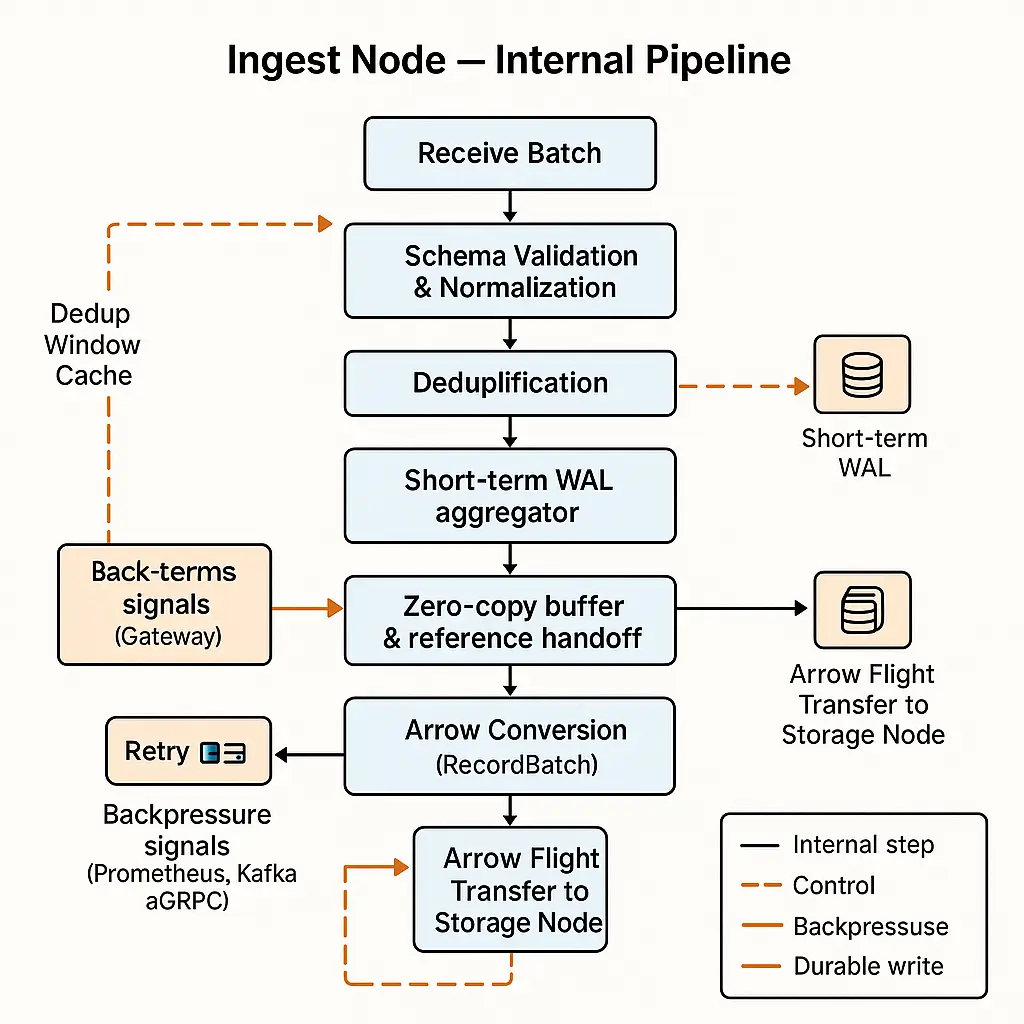
The Ingest Node is a central piece in Openwit’s pipeline – it’s responsible for taking the batch of events from the gateway and preparing it for long-term storage. Several important things happen in the ingest node:
High-Throughput Processing with Zero-Copy: When the ingest node receives a batch, it processes it using an actor (a lightweight concurrent task). One important performance technique used here is zero-copy data transfer. Instead of making copies of the data for every stage (which would be memory and CPU-intensive), the ingest node passes around references to the original batch data. In practice, this might mean using shared memory pointers or reference-counted buffers so that multiple parts of the code can work with the same data without duplicating it. This keeps memory usage lower and speeds up processing (especially critical when dealing with large batches of logs or metrics).
Deduplication of Data: Openwit has a mechanism to avoid ingesting duplicate data points within a certain time window. For example, imagine a situation where the same log event might be sent twice due to a retry or error upstream. The ingest node keeps a short-term cache (or fingerprint) of recently seen data (based on timestamps and perhaps a hash of the content). If a new incoming record is exactly identical to one seen in the last, say, 1 hour (the time window can be configured), the system can recognize it as a duplicate and skip or ignore it. This deduplication ensures that during bursts or error conditions, you don’t store the same data twice, which saves storage and prevents skewed query results. It’s especially useful for metrics, where duplicate sends could incorrectly amplify a value, or for logs where replays could occur. By doing this at ingest, Openwit ensures the data set remains clean and unique.
Write-Ahead Logging (WAL): Short-term and Long-term: After preparing the batch (and ensuring it’s unique), the ingest node writes the data to disk in a Write-Ahead Log (WAL). Write-Ahead Logging is a standard technique for ensuring data durability: you append incoming data to a log on disk so that if anything crashes or goes wrong downstream, you have a record of what was received and can recover from it. Openwit actually uses two layers of WAL:
- Short-term WAL: This is a rapid log of recent batches. Each batch that comes in is written to the WAL file (or files) immediately. Only once this write is successful does Openwit consider the data “ingested”. For example, if data came from Kafka, Openwit will only commit the Kafka offset (acknowledging that the message has been processed) after writing to the WAL. This guarantees that if the system crashes after reading from Kafka but before saving, it won’t lose data – Kafka will simply resend it because the offset wasn’t committed. The short-term WAL files are kept relatively small (maybe aligned with batch sizes). They serve as the first line of defense in case of a crash or shutdown.
- Long-term WAL: In addition to the immediate log, Openwit maintains a more aggregated WAL for longer-term durability. The system will group the smaller WAL entries (perhaps by time intervals, e.g., hourly or daily) into larger long-term WAL files. The purpose of this is twofold: one, it’s easier to manage or replay data from a single large file per day than thousands of tiny batch files; and two, it can be used for bulk recovery or re-indexing operations. For instance, if down the line you needed to rebuild an index or restore a dataset, you could use the long-term WAL files as the source of truth for a given day’s data. Essentially, the long-term WAL is an archive of what’s been ingested in chronological chunks, whereas the short-term WAL is a real-time journal ensuring immediate durability.
Metadata in Postgres (Source of Truth): As soon as a batch is successfully written to the short-term WAL (meaning the data is safely on disk), Openwit records metadata about that batch in a PostgreSQL database. This Postgres instance acts as a metadata catalog or source of truth for all ingested data. Entries might include:
- Batch/WAL identifier
- The time range of data in that batch (the earliest timestamp and the latest timestamp in the batch)
- Size (number of records, bytes),
- Perhaps a pointer to the WAL file location or offset
- Other metadata (like which node processed it)
This metadata is crucial for later stages: it’s used during querying to know what data exists where. It’s also useful for monitoring the system’s progress. By having this in a relational DB (Postgres), Openwit makes it easy to query or update this metadata as needed (and Postgres is a robust, proven store for such information).
At this point in the flow, the data is safely persisted (in WAL and recorded in metadata). This means we can confidently say “we have the data” and acknowledge to sources like Kafka that it’s been ingested. The next concern is moving this data to long-term storage and making it queryable. Openwit begins this by converting the data to a columnar format and sending it off to a storage node.
Forwarding to Storage (Arrow Conversion): Inside the ingest node, once the WAL write is done, an actor (or background task) takes the batch of data and prepares it to send to the storage layer. This involves converting the batch (which is likely still in a JSON or row-based structure at this point) into an Apache Arrow columnar format. Arrow format organizes the data by columns in memory, which is ideal for analytic queries and also needed for efficient creation of Parquet files (since Parquet is a columnar on-disk format).
By converting to Arrow once here, the system can stream those Arrow record batches to the storage node over Arrow Flight (as mentioned in the communication section). The use of Arrow here also enables the zero-copy transfer – instead of serializing each record, the entire batch (already in an efficient binary format) can be sent over the network. The ingest node essentially says, “here’s a batch of Arrow data representing these 1000 log events,” and the storage node will receive that in the same representation.
To summarize this stage: the ingest node ensures data durability and cleanliness (via WAL and deduplication), and then hands off the data in a format suitable for storage and fast querying. Now let’s look at what the storage node does with it.
Storage Node and Cloud Storage (Parquet Files)
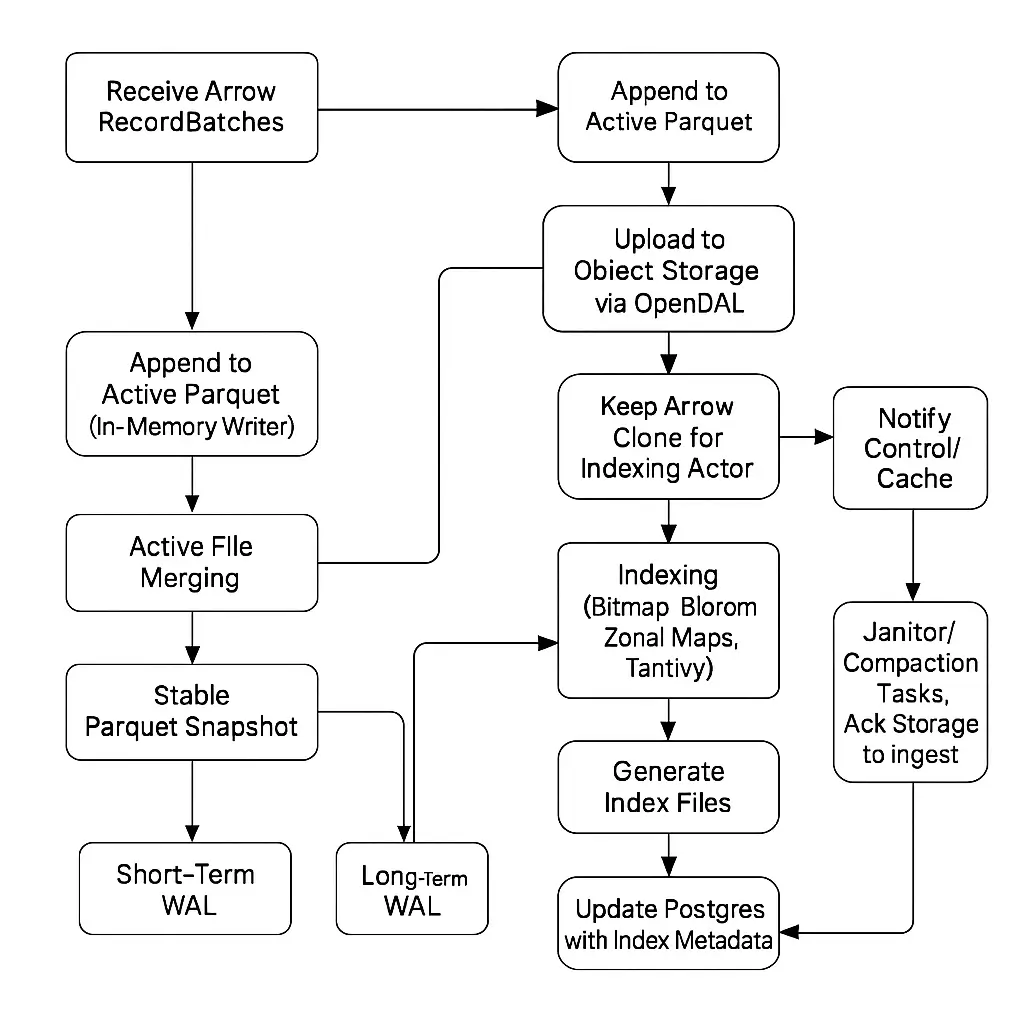
The Storage Node is where data gets packaged for long-term retention and made ready for querying. It’s responsible for turning the stream of incoming Arrow batches into files on disk and eventually in cloud storage. Here’s what happens on the storage node:
Receiving Arrow Batches: The storage node receives the Arrow-formatted batch of data from the ingest node (via Arrow Flight). At this stage, the data is in memory on the storage node in a nice columnar structure.
Parquet File Creation (Active vs Stable Files): Openwit stores data in the Parquet format for long-term (Parquet is a columnar, compressed file format very well suited for analytics). However, it doesn’t just immediately dump each incoming batch as its own Parquet file; that would result in tons of tiny Parquet files which is not efficient for later reading. Instead, the storage node accumulates data into larger Parquet files. It uses a two-phase approach with active and stable files:
- An Active Parquet file is where incoming data is first written. Think of this as the currently “open” file that new batches are appending to. As each Arrow batch comes in, the storage node writes it to the active Parquet file (converting the Arrow in-memory data into Parquet on disk).
- In parallel, a Stable Parquet file is being built as a slightly lagging copy of the active one. The stable file will only be finalized once it reaches a configured size (which you set in the config, e.g., you might want final Parquet files to be, say, 100 MB or 1 GB for optimal query performance). The stable file lags the active file, meaning it might not include the absolute latest batches until it’s ready. The benefit of this two-file approach is efficiency:
- If you had only one file, to keep appending new Arrow data, you might have to repeatedly read and rewrite the file (because Parquet files are optimized for big, sequential writes rather than continuous appends). That would be costly.
- With an active file that’s small and being actively written, the system can flush data quickly. The stable file can periodically take a snapshot of the active file’s data (since Parquet is append-friendly up to a point) without interrupting the active writes too much.
- Once the stable file has accumulated enough (it has “caught up” to the active file data and reached the target size), the stable file is closed/finalized. At that moment, the active file might still continue on with new data (perhaps by then, the active file was reset to start accumulating the next chunk).
In summary, active files handle the immediate incoming stream, and stable files are used to consolidate that stream into nice chunked Parquet files of the right size for efficient storage and retrieval.
Uploading to Cloud (Cold Storage): When a stable Parquet file is complete (i.e., it hits the desired size or time partition), it’s ready to be shipped off to long-term storage. Openwit uses OpenDAL (an open-source data access layer) to interface with cloud storage. In the typical setup, this will be an Azure Blob Storage container (though OpenDAL can abstract many storage backends, so it could be other cloud storage or even local/NFS, depending on config). The storage node will upload the Parquet file to the cloud – effectively, this means the data is now durably stored in a central repository, accessible to other nodes for querying.
- The use of cloud object storage (like Azure Blob) means Openwit treats storage in a “data lake” style: decoupling compute from storage. This allows nearly infinite scalability of storage (just add more files in the blob store) and cost-effective retention (cloud storage is cheaper than keeping everything on local disks of search nodes, for example).
Metadata Recording: Just like with ingestion, when a Parquet file is uploaded, the system records metadata about it in Postgres (the metadata catalog). It will update or insert entries that describe:
- The file’s location (e.g., a URI or path in the cloud storage)
- The size of the file
- The time range of data it contains (this is very important for query pruning later – if a query asks for data from October 10, 2025, the system can look up which files cover that date range)
- Perhaps a file ID or partition ID
- A flag that it has been uploaded (so it’s now safe in cloud storage).
Additionally, Openwit can use this metadata for time-based data retention policies. For example, if you decide to prune (delete) data older than X days, it would consult these entries to find which files (and their indices, see below) to remove from cloud storage. By logging the start and end timestamps of each file, such maintenance operations become feasible.
Initiating Indexing: After the Parquet file is successfully stored, the storage node doesn’t sit idle – it starts the indexing process for that data. Internally, an actor on the storage node keeps a copy (or reference) of the Arrow data or can read the Parquet back immediately, and now it spawns an indexing actor to create indexes (we’ll detail indexing in the next section). Importantly, indexing is performed after the file is safely in cloud storage, decoupling ingestion speed from indexing. This way, writing data is not slowed down by the perhaps more CPU-intensive task of building indexes – indexing can happen asynchronously.
At the end of the storage node’s process, the data is:
- Stored in cloud as a Parquet file (long-term, cold storage).
- Logged in metadata for future reference.
- Set to have indexes built for it to accelerate queries.
All these steps ensure that by the time data leaves the storage node, it’s query-ready and safely stored. Now let’s dive into what indexing means in Openwit and how it works.
Indexing Data for Fast Queries
While Parquet files are great for compact storage and analytical scanning, queries can be even faster if the system has indexes to quickly narrow down the search. Openwit supports multiple indexing strategies to optimize query performance, especially given the mix of data types (logs with text, metrics with numeric values, etc.). The indexing occurs on the storage node (after data is uploaded to cloud, as mentioned):
Why Index? Think of an index as a shortcut to find relevant data without scanning everything. For example, if you have 1 TB of log data and you want logs where error_code = 500, a suitable index could tell you exactly which file segments might have error_code 500 without reading all 1 TB. This dramatically reduces query times.
Types of Indexes Supported: Openwit’s eventual goal is to support many types of indexes so users can choose what fits their data. Currently, the system includes:
- Bitmap Indexes: These are ideal for discrete fields with not too many unique values. A bitmap index is essentially a mapping of values to bitmaps indicating which rows (or blocks of rows) contain that value. For example, for a field like status_code in logs (which might have values 200, 404, 500, etc.), a bitmap index can quickly identify all entries with status 500 by looking at a bitmap (where a 1 in position i means “row i has status 500”). Bitmaps are extremely fast for filters and take very little space when the number of distinct values is limited.
- Bloom Filters: A Bloom filter is a probabilistic data structure that can quickly test if a value might be present or is definitely not present in a dataset. Openwit can maintain bloom filters on certain fields per data chunk. For instance, you could have a bloom filter for the set of all user IDs present in a file; then at query time if you’re searching for a particular user ID, the bloom filter can instantly tell you if that file cannot possibly have that ID (thus you can skip it) or if it might (in which case you need to scan it). Bloom filters are very fast and memory-efficient, though they can have false positives (they might say “maybe it’s there” when it’s not, but never miss a true presence). They are great for high-cardinality fields to avoid scanning unrelated data.
- Zone Maps (Min/Max Indexes): A zone map stores the minimum and maximum value of a field for each block of data (for numeric or timestamp fields usually). For example, if a Parquet file is internally divided into row groups (blocks of a few thousand rows), a zone map for the timestamp field might store the earliest and latest timestamp in each block. At query time, if you are looking for data in the time range 10:00-11:00, any block whose min-max timestamp range doesn’t overlap that interval can be skipped entirely. Zone maps are simple but effective for pruning based on ranges (especially time, which is a common filter in observability queries).
- Full-Text Index (Tantivy-based): Logs often contain unstructured text (log messages, error descriptions, etc.) where you want to do keyword searches (e.g., find all logs that contain the word "timeout"). For this, Openwit integrates with Tantivy, which is a full-text search engine library (akin to Lucene, but in Rust). Tantivy can build an inverted index of terms for textual fields. If Openwit is configured to index a “message” or “description” field of logs, it will create Tantivy indices that allow lightning-fast text queries. For example, searching for "error" or complex text patterns can be resolved by looking up the term in the inverted index rather than scanning every log message.
- (Future) Other Index Types: The architecture is open to adding more index types (for instance, geospatial indexes if needed, or more advanced time-series indexes for metrics). The user can configure which indexes they want based on the data and query patterns. Each index type adds some overhead to create and store, but yields faster queries for certain query types. Openwit’s goal is to let you customize this trade-off.
Index Creation and Storage: When the indexing actor runs for a newly uploaded Parquet file:
- It reads the data (either from the Arrow batch it kept or directly from the Parquet file) and builds the chosen indexes.
- Each type of index might result in separate index files/artifacts. For example, a Tantivy index for text could be a set of files (posting lists, term dictionary, etc.), a bloom filter might be a small binary blob, bitmaps could be stored as bitset files, etc.
- Once built, these index files are also uploaded to the cloud storage, alongside the data file. (They could be in a parallel path or bucket, e.g., for a data file
logs_2025-10-16_01.parquet, you might have an index filelogs_2025-10-16_01.bloomandlogs_2025-10-16_01.tantivy, etc.) - The metadata in Postgres is updated to include references to the index files. Openwit will note that for the given Parquet file (or partition of data), there are indexes of types A, B, and C available and where to find them in storage.
Using Indexes: (This will be further explained in the query section, but it’s worth noting context here.) Once the indexes are in place, any queries that come in can leverage them. For example, if a query has a WHERE clause filtering on a field that has a bitmap or bloom index, the search node can fetch that index instead of scanning the whole file. If the query has a full-text search keyword, the search node can consult the Tantivy index to get candidate results without reading all logs. Indexes drastically reduce the amount of data that needs to be read from disk or cloud for answering queries, which is why Openwit can achieve fast response times even with huge volumes of data.
To sum up, indexing is what makes Openwit stand out compared to many classical OLAP solutions. It’s not just blindly scanning everything – it actively builds smart indexes to accelerate queries, all while storing data in an efficient columnar format. With data safely stored and indexed, the last major piece of the puzzle is how queries are executed and how the system uses all these pieces (cache, indexes, metadata) to return answers quickly.
Query Processing and the Search Node
When you want to retrieve data or get insights from Openwit, you typically issue a query (often an SQL query given Openwit’s OLAP nature). The Search Node is in charge of taking that query and producing results. Here’s how the query processing works, step by step:
- Receiving a Query: A user or application sends a query (for example, an SQL SELECT statement filtering logs by some criteria and time range, or a query to compute an aggregate over metrics). In a distributed setup, this query might go to a Proxy Node first, which then forwards it to one of the Search Nodes. In a monolithic setup, the single node just takes it directly. For clarity, let’s assume it’s now at a search node ready to execute.
- Planning the Query: The search node parses the SQL query and turns it into an execution plan. Openwit uses Apache DataFusion as its primary query engine. DataFusion is a powerful query planner and executor that operates on Arrow data. It can optimize the query (reorder filters, push down predicates, etc.) and will be able to execute it in a parallel/distributed fashion (with Ballista, which is DataFusion’s distributed execution framework, the query can run across multiple nodes if needed). For example, if your query says
SELECT count(*) FROM logs WHERE level = 'ERROR' AND timestamp BETWEEN X and Y, DataFusion will create a plan that involves reading relevant data files, filtering for level = 'ERROR' and the time range, then counting. - Cache Check (Short-Circuit if Possible): Before pulling lots of data from storage, Openwit checks whether the needed data is already available in the Cache Nodes:
- Recall that Cache Nodes may hold popular datasets either in memory or on local disk (parquet files already downloaded).
- The search node will determine the time range and possibly other identifiers of data that the query needs (using the WHERE clause or the FROM clause if data is partitioned by time).
- If it finds that a cache node has all the required data for that range (for example, the cache has the Parquet files or in-memory batches for October 16, 2025, and that’s exactly what the query is asking for), then the search node can offload the query to the cache node or retrieve the data directly from the cache node.
- In practice, the search node might send the execution plan (or a portion of it) to the cache node. The cache node, which can also run DataFusion, will scan its local data (RAM or disk) instead of going to cloud storage, execute the query plan, and return the results. This is much faster than downloading from the cloud and also alleviates the load on the network/storage layer.
- If the cache only has part of the data needed (say half the data range is cached), the system could use what’s in cache for that portion and fetch the rest – but for simplicity, let’s assume either it’s a cache hit for all or we move to fetching from the cloud.
- Fetching Metadata & Index Info: If the query cannot be fully answered by cache (cache miss or partial), the search node has to gather the data from cold storage. It doesn’t blindly start downloading everything; instead it uses the metadata and indexes we discussed:
- The search node will query the Postgres metadata store to find which Parquet files (or data partitions) contain data for the query’s timeframe and conditions. Since each Parquet file upload was logged with its time range, this step immediately narrows down the list of candidate files. For example, if you ask for data in Oct 2025, the system won’t waste time on files from Sept 2025 or Nov 2025.
- The metadata also tells it where those files are (e.g., which cloud path).
- Importantly, the metadata entry for each file also lists what index files are available for it. The search node will then fetch the relevant index files from cloud storage first (these are much smaller than the data files).
- By loading the indexes (like bloom filters, zone maps, etc.) into memory, the search node can perform pruning:
- For each candidate Parquet file, check the indexes to see if the file actually might have data matching the query filters. For instance, if the query is
WHERE level = 'ERROR', and a particular file has a bitmap index forlevelthat shows it has no 'ERROR' entries (only 'INFO' and 'WARN'), that file can be skipped entirely. - If the query had a text search component (say,
message CONTAINS 'timeout'), the search node can use the Tantivy full-text index for each file to get a list of matching entries or to see which files contain the word "timeout". If a file’s Tantivy index indicates zero hits for "timeout", again that file can be skipped without reading it. - Zone maps can be used here too (e.g., skip files or parts of files where timestamps are out of range, although ideally we wouldn't have retrieved those out-of-range files in the first place due to the time partitioning logic).
- For each candidate Parquet file, check the indexes to see if the file actually might have data matching the query filters. For instance, if the query is
- After applying indexes, the search node will have a refined list of which Parquet files actually need to be read to answer the query.
- Data Retrieval from Cloud: For the remaining relevant Parquet files (the ones not eliminated by indexes), the search node (or potentially multiple search nodes working in parallel as part of Ballista) will download those Parquet files from cloud storage. Thanks to the earlier steps, this is likely a much smaller set of files than the total, making the download overhead manageable. OpenDAL is used behind the scenes to fetch the files from Azure (or the configured storage), possibly reading streams if supported.
- Query Execution (DataFusion & Ballista): With the needed Parquet data in hand (either now on local disk or in memory after reading), DataFusion takes over to execute the query plan:
- The Parquet files are scanned using DataFusion’s Parquet readers (which leverage vectorized processing – very fast in-memory operations on Arrow format).
- Filters (WHERE clauses) that weren’t fully handled by indexes are applied at this scan stage to drop any non-matching records.
- If multiple search nodes are involved (for example, if the query was distributed across nodes for parallelism), each will process a portion of the data (maybe each took a subset of the files or partitions). Ballista coordinates this, and there might be a shuffle stage if needed (for aggregations, joins, etc., intermediate results might be exchanged among nodes).
- The query may involve aggregations (like COUNT, SUM) or joins or other SQL operations. DataFusion will handle those using its in-memory compute capabilities.
- The end result of the execution is the answer to the query (could be an aggregated result, or a set of records that match).
- Returning the Results: Finally, the search node (or coordinating node) sends the results back to the client that asked the query. Despite all the complex steps under the hood, this entire process is optimized to be as fast as possible. Openwit aims to achieve sub-second query responses for most interactive queries, even with very large datasets. Of course, exact performance depends on how much data needs scanning, but by using caching and indexing to minimize work, Openwit’s architecture is designed to avoid the typical slowdowns one might see in naive systems.
- Caching Results (if applicable): Optionally, Openwit can also use the cache nodes to store recently accessed data or results. For example, if a particular query (or time range) is repeatedly accessed, the system could keep those Parquet files on a cache node or keep the Arrow in memory, anticipating that future queries will hit the cache. This isn’t an explicit step in the query execution, but it’s part of the overall strategy to continually improve performance for hot data.
A quick note on full-text search integration: Since DataFusion is geared towards structured data and SQL, when a query includes full-text conditions (like searching within log messages), the search node will rely on Tantivy indexes to fulfill that part. In practice, the search node might retrieve from Tantivy a set of document IDs or offsets that match the text condition, and then use that as a filter on the Arrow data. This way, you get the power of full-text search combined with analytical queries (something not common in traditional OLAP databases).
Caching and Tiered Storage for Speed
We touched on caching above, but it’s worth elaborating how Openwit’s caching works and how data is tiered across storage types (because this is a big part of how Openwit becomes faster and more efficient over time or under heavy use): Openwit’s storage is tiered into essentially three layers, which we can analogously call:
Cold Storage (Cloud): Also nicknamed Cryo store (like “cryogenic” for cold). This is the Azure Blob or cloud object storage where all data ultimately resides. It’s durable and cost-effective, but relatively slow to access (due to network latency and bandwidth limits).
Hot Storage (Disk Cache): Nicknamed Pyro store (pyro = fire = hot). This is typically the local disk (SSD) on a cache node. Frequently needed Parquet files can be kept on disk in the cluster so that queries can read them locally rather than pulling from the cloud each time. Disk access (especially SSD) is much faster than cloud, and it avoids repeated download costs.
Ultra-Hot Storage (In-Memory Cache): Nicknamed Electro store (electric = very fast). This is data stored in RAM as Arrow record batches on cache nodes. RAM access is orders of magnitude faster than even an SSD disk. The trade-off is that you can’t store as much in RAM, so usually only the most important or recent data is kept here. This is great for real-time dashboards or frequent queries on the latest data – you can get an instantaneous response because the data is already sitting in memory, ready to go.
How the cache is used: The system allows deploying one or more Cache Nodes whose job is to pull data from the cloud and hold it at these faster tiers. You (as the user or admin) can configure policies for what to cache. For example:
- “Cache the last 7 days of data on disk and the last 1 hour of data in memory” might be a policy for metrics if you often query recent data.
- Or you might specify certain key datasets or index files to keep in cache if you know queries will repeatedly touch them.
When a query comes in, as described, the search node first checks these caches. Over time, as queries run, the cache nodes might also automatically retain data that was accessed (thus anticipating future accesses might hit the same data).
The cache nodes also participate in query execution (they have the same query engine capability), so they can fulfill queries independently if they have the required data. This tiered approach means Openwit can efficiently serve both recent data (likely cached) and older data (from cold storage), adjusting the strategy based on what’s requested.
For the user, this is largely transparent – except you notice that queries for frequently accessed data become faster (because behind the scenes it’s now served from a hotter tier). It’s similar to how a content cache on the internet speeds up web page loads after the first time – here it’s speeding up data access for queries.
Key Advantages and Differentiators of Openwit
By now, you’ve seen how Openwit is constructed and how data flows through it. Let’s highlight how it is different from other solutions and what advantages these design choices bring:
Unified Observability Platform: Openwit isn’t just a metrics database or just a log search system – it’s built to handle logs, metrics, and traces in one unified way. Traditionally, organizations might use separate tools for each (like a time-series DB for metrics, an ElasticSearch cluster for logs, etc.). Openwit’s unified approach means you can correlate and store all these data types together, simplifying your architecture and potentially reducing duplication of effort.
Flexible Deployment (Scale Up or Out): The ability to run monolithically or in a distributed cluster means Openwit can cater to different scales. You can start small (even just one server running everything for a dev environment) and later split out components to scale horizontally for production. Many legacy solutions force one or the other (either not scalable past one node, or overly complex even for small cases); Openwit gives you both options.
Actor-Model Concurrency in Rust: Under the hood, Openwit’s use of an actor system (a programming model where components are isolated, communicate by messages, and handle tasks asynchronously) allows it to process massive concurrent workloads without blocking. This design (along with Rust’s performance and safety) means it can ingest and handle data with minimal downtime and high resilience. If one actor (say an indexing task) fails, it doesn’t crash the whole system – it can be isolated and restarted by the supervisor logic in the actor system. This leads to a robust system that can self-heal certain issues and utilize multi-core hardware very efficiently.
Optimized Communication (Gossip + gRPC + Arrow Flight): Openwit’s nuanced approach to inter-node communication avoids the pitfalls of a one-size network layer. Gossip ensures cluster state sync with negligible overhead (no central bottleneck for heartbeats). gRPC ensures reliable and structured communication for control commands. Arrow Flight turbocharges data transfer, making it possible to move large volumes (gigabytes) of data quickly between nodes. The net effect is a system that maintains coordination and data flow at high speed, which is crucial for real-time analytics on big data.
Schema Enforcement and Data Quality: Unlike some schemaless log stores, Openwit enforces a schema at ingest time. This is advantageous because it keeps your data consistent and clean. Queries don’t fail due to type mismatches, and you won’t get confusing results from inconsistent field usage. It might require a bit more upfront definition, but it saves a ton of headache later on. Also, by rejecting or normalizing bad data early, Openwit ensures that only high-quality data is stored and analyzed.
High Throughput Ingestion (Batch + Zero Copy + WAL): The ingestion pipeline is built for speed and safety:
- Batching reduces overhead, so the system can ingest tens of thousands of events per second with ease.
- Zero-copy processing means minimal CPU wasted on moving memory around – more CPU goes to actual transformation and compression rather than overhead.
- The dual WAL strategy provides strong durability guarantees (comparable to enterprise databases) – data is never acknowledged until safely on disk, and there’s always a recoverable log. This is a big plus for reliability; even in the face of crashes, you can recover what was in flight.
- Deduplication at ingest prevents system overload from duplicates and ensures correct metrics (especially important in exactly-once processing scenarios or when upstream retries happen).
Columnar Storage (Parquet) with Cloud Scalability: By using Parquet on cloud storage, Openwit effectively implements a data lakehouse architecture for observability data:
- Columnar storage means queries (especially analytical ones that only hit a few columns) run faster and storage is efficient (column compression).
- Storing in cloud object storage means you’re not limited by the disk size of any cluster node – you can retain as much data as you want cost-effectively. It also decouples storage from compute: you can shut down parts of the cluster to save cost (if not querying) without losing the data, since it lives in durable storage outside.
This approach differs from traditional monolithic databases which keep all data on local disks and might need costly expansion to add storage. Openwit can leverage cloud for virtually unlimited storage.
Sophisticated Indexing: Openwit doesn’t rely only on brute-force scanning. The variety of indexes (bitmap, bloom, zone map, full-text) is a major differentiator. It means Openwit can handle:
- Structured filtering (e.g., metrics or logs by service, status, user) extremely fast via bitmaps and blooms.
- Time range queries quickly via zone maps and time partitioning.
- Keyword searches in log text via Tantivy full-text indexing, which many columnar databases can’t do efficiently since they aren’t built for text search.
- And since indexes are configurable, you can tune the system: if you have a field that’s commonly filtered on, you add an index for it to speed those queries. This gives Openwit an edge in query performance for a broad set of query patterns. Many observability tools either choose full-text search but sacrifice analytical queries, or vice versa; Openwit strives to excel at both by combining indexing with OLAP.
Intelligent Query Execution: Using Apache DataFusion means Openwit benefits from a modern query engine capable of distributed execution and SQL optimization. The integration of Ballista allows scaling out query processing across multiple search nodes (massively parallel processing for big queries). This is similar to how big data SQL engines (like Spark, Druid or ClickHouse cluster) work. In addition, by integrating the index usage into the query planner (pruning data before reading) and leveraging cache, Openwit’s query engine does as little work as necessary to get the answer. The aim is to achieve sub-second responses on indexed queries and generally interactive performance for large-scale data analysis.
Multi-Tier Caching: The presence of cache nodes and tiered storage is a big plus for real-world usage:
- It reduces latency for frequent queries (as data is served from memory or local disk, which is much faster).
- It reduces cost and load on the cloud storage (fewer repeated downloads of the same file, which can incur cloud egress fees and use bandwidth).
- It provides a buffer against outages – if the cloud storage has a hiccup, you might still have recent data in cache to serve queries.
- Many traditional systems lack this or leave it to the user (for example, you’d manually script caching or rely on the OS disk cache). Openwit builds it into the system design.
Resilience and Fault Tolerance: With the control node monitoring the cluster (and using gossip for failure detection), and with WAL + metadata ensuring recoverability, Openwit is designed to handle node failures gracefully. If an ingest node dies, another could replay the WAL from the cloud or the long-term WAL to catch up. If a search node fails mid-query, the query could be retried or run on another node. Gossip ensures everyone knows about the failure quickly, and the control node can redirect traffic as needed. This kind of self-healing property is crucial in distributed systems and is an advantage Openwit has by design (inspired by battle-tested systems like Cassandra, which also uses gossip and hinted handoff, etc.).
Designed for Observability Needs: Unlike a generic database, Openwit’s features (schema enforcement, time-based partitioning, mixing text search with analytics, multiple ingest methods, etc.) are tailored to logs, metrics, and traces. It knows, for example, that time is a primary dimension (and thus everything is organized by time for efficient slicing). It knows that logs benefit from full-text search, while metrics benefit from compression and fast aggregations. By handling these within one system, Openwit provides a one-stop solution for observability data that traditionally required a Frankenstein combo of tools (Prometheus + ElasticSearch + some tracing tool, glued together). This specialization makes it more efficient and easier to use for DevOps/SRE teams who can rely on one system with one query interface (SQL) to ask complex questions that span across metrics, logs, and traces together.
In essence, Openwit’s differences and advantages come from blending the best of several worlds: stream processing techniques (for ingest), database techniques (for storage and indexing), search engine techniques (for text indexing), and cloud-native design (for scalability and durability). It’s a cutting-edge approach aimed at handling today’s high-volume, high-variety observability data with speed and grace.